Enhancing Flow Separation through Fidelity Pointwise

Airplanes and thus aircraft wings have gained quite some attention from researchers in recent times owing to their significance in our life and the potential impact of developments in this area, on reducing carbon footprint and making air transportation more environmentally friendly.

Centered around this theme is the current study on how to improve lift generated by aircraft wings at lower angles of attack and delaying stall. One of the mechanisms used for this purpose is the injection of fluid (air) from the wing, into the oncoming flow. This adds momentum to the flow going above the airfoil, thus helping the flow overcome stall at that angle of attack due to lack of momentum.

The flow past an asymmetric airfoil is studied using steady-state, turbulent (RANS) simulations, in an incompressible flow field. Different simulations were performed to check the influence of the position of the slot from where mass is injected into the flow, the angle at which the injection happens, the flow rate of the injecting fluid, and to compare the improvement in lift against the corresponding airfoil without mass injection. Meshing the region near the area where the injected fluid meets the oncoming flow is quite important but challenging. The presence of the small slot at an angle poses a challenge to the typical O-grid, C-grid or H-grid approaches.

This article helps understand the features in Fidelity Pointwise which help generate improved meshes for such cases where it is difficult to get a good mesh in complex geometric scenarios using built-in meshing tool in commercial solvers.

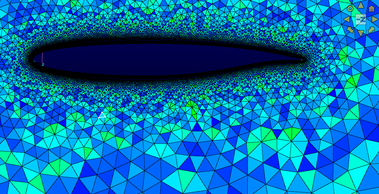
Figure 1. Mesh generation using Fidelity Pointwise

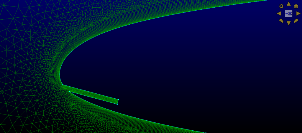
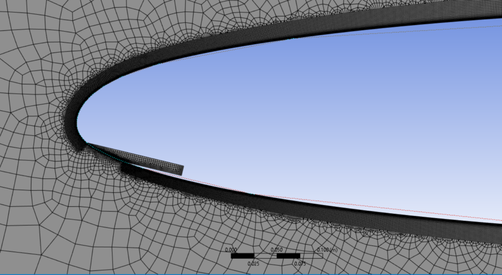
Fig. 1 represents a mesh generated using Fidelity Pointwise on the same geometry. Fig. 2 represents the baseline mesh [1], zoomed close to the region mentioned above. At first glance, it is immediately visible that using Fidelity Pointwise unique TRex mesh generation algorithm, it is possible to obtain a much smoother transition from the boundary layer mesh to the mesh in the free-stream region. The algorithm also give you control over smoothing parameters which help obtain better quality meshes and smoother transition in hybrid meshing. Furthermore, the generation of the mesh (and re-meshing, when a few spacings/divisions are modified) is faster when using Fidelity Pointwise.

Figure 2. Mesh generated with another built-in mesher in a commercial solver[1]

Mesh quality analysis

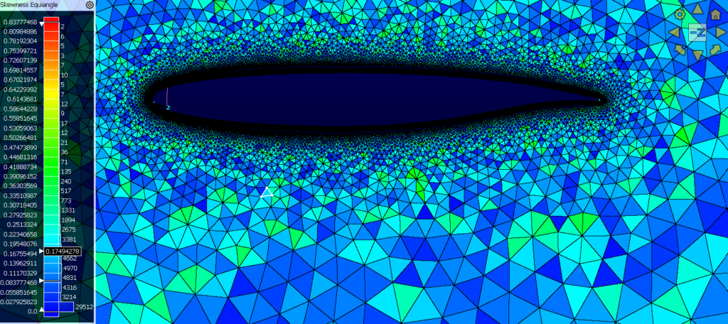
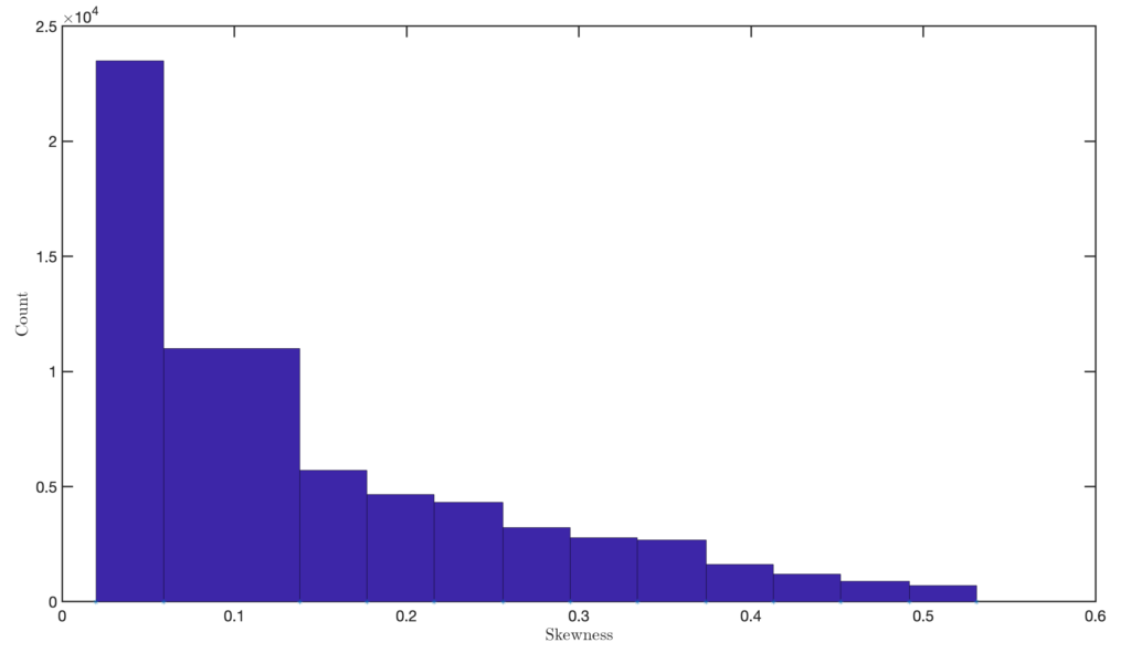
Proceeding to the analysis of the generated mesh, Fidelity Pointwise offers a wide range of parameters to evaluate mesh quality. One key parameter is skewness, which measures how much a cell deviates from an ideal shape (e.g., equilateral or orthogonal). High skewness values can negatively affect the accuracy and stability of a CFD simulation, as skewed cells can introduce numerical errors and compromise convergence. Fig. 3 shows the skewness distribution of the mesh generated using Fidelity Pointwise. It is also possible to check the skewness of a particular element (highlighted in yellow in the picture) by clicking on it, with the corresponding skewness value displayed on the color bar to the left.

Figure 3. Skewness distribution of the mesh generated using Fidelity Pointwise

Figure 4. Skewness distribution of the mesh generated with another built-in mesher in a commercial solver[1]

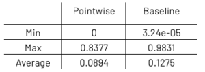
For comparison, Fig. 4 presents the skewness distribution of the mesh generated using a common commercial solver meshing tool [1]. Additionally, Fidelity Pointwise provides the option to export this mesh metric distribution to a CSV file, allowing for further detailed analysis.

The percentage variation in the average skewness w.r.t. the Fidelity Pointwise mesh is around 42% while the variation in the maximum is around 17%, indicating that higher fraction of the elements have lower skewness.

CAE export

Fidelity Pointwise provides the option to select a CAE solver which would later be used for performing the simulations. This would provide the option to export the mesh file in the appropriate format as required by a range of CAE solvers, and also set boundary conditions during the meshing itself. You can find the full list of CAE solvers supported by Pointwise here.

But how do these changes in the mesh affect the results?

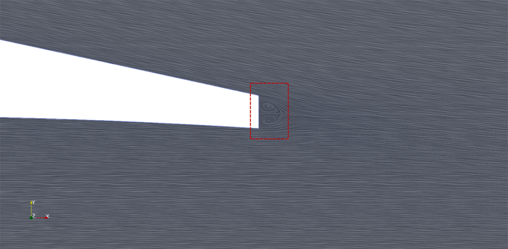
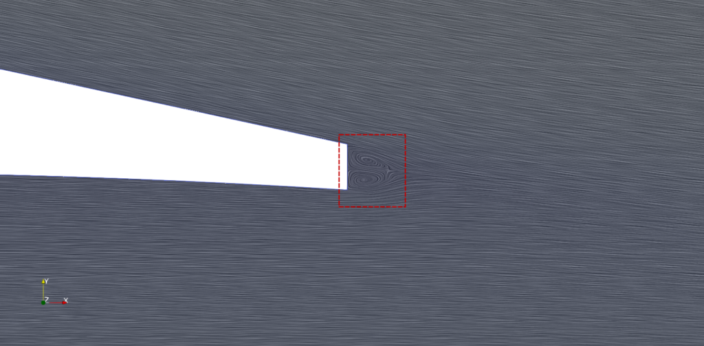
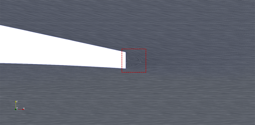
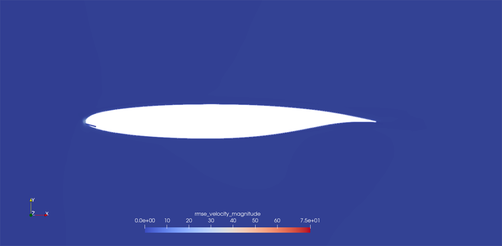
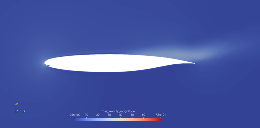
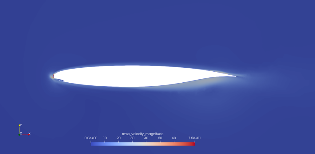
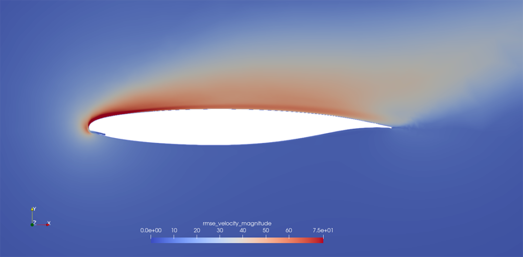
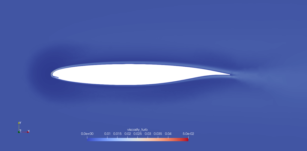
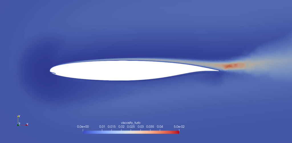
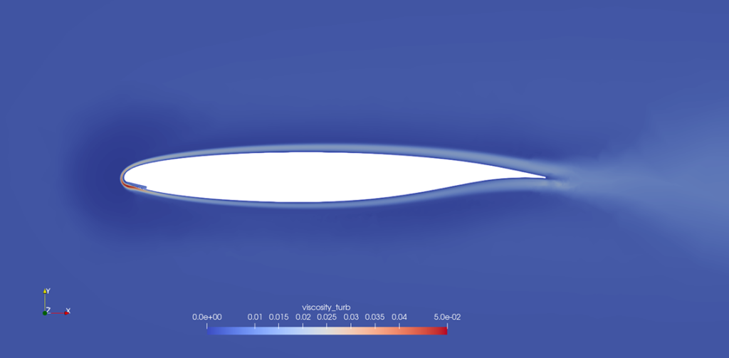
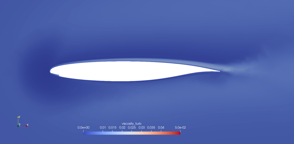
The simulation was performed using the k − ω SST turbulence model, with standard air properties, at a Reynolds number of 10⁷. The convergence criterion was set to 1e-06 for all the quantities. The analysis of lift and drag coefficients as obtained from both the meshes show variation within an acceptable range (< 4%) for both parameters at 0^o angle of attack (AoA). However, at higher AOA (16^o), close to the stall angle, the differences in the predictions differ significantly. The relative difference in prediction of lift and drag coefficients is 11.44% and 19.72% respectively, w.r.t. the baseline mesh. The prediction of such different values of forces can be attributed to the differences in the flow field obtained from the two meshes. Figures 5, 7, 6, 8, 9, 11, 10, 12 illustrate the differences in the flow fields between the two meshes. These images include LIC (Line Integral Convolution) plots of the flow field, as well as RMSE (root-mean-square error) of the velocity magnitude and turbulent viscosity at 0o and 16o AoA. While the differences at AoA = 0o are minor, they become much more pronounced at AoA = 16o, near the stall angle, where the flow physics becomes increasingly complex.

Figure 5. Improved mesh with Fidelity Pointwise – 0^◦ AOA

Figure 6. Improved mesh with Fidelity Pointwise – 16^◦ AOA

Figure 7. Baseline Mesh – 0^◦ AOA

Figure 8. Baseline Mesh – 16^◦ AOA

Figure 9. Improved mesh with Fidelity Pointwise – 0^◦ AOA; RMSE of velocity magnitude

Figure 10. Improved mesh with Fidelity Pointwise – 16^◦ AOA; RMSE of velocity magnitude

Figure 11. Baseline Mesh – 0^◦ AOA; RMSE of velocity magnitude

Figure 12. Baseline Mesh – 16^◦ AOA; RMSE of velocity magnitude

A key factor contributing to the improved performance of the Fidelity Pointwise mesh is the smooth transition in aspect ratios, which is not present in the mesh generated by the built-in mesher of the commercial solver. In cases like these, it is crucial to carefully match the inflation layer thickness, boundary layer thickness, and the size of neighboring cells outside the inflation layer. Failure to do so can force the boundary layer to artificially fit within the inflation layer, leading to spurious patterns of turbulent viscosity.

The RMSE of the velocity magnitude, which indicates fluctuations or errors in the flow field, is notably lower and confined to a smaller spatial region in the Fidelity Pointwise mesh compared to the mesh generated by the built-in mesher. Since this simulation is a steady-state RANS case, the RMSE is calculated on the solution at various iterations prior to convergence. These plots highlight better convergence of the flow field when using the Pointwise mesh, further demonstrating its superiority over the built-in mesher in this scenario.

Furthermore, using Fidelity Pointwise, the mesh generation process was more tractable, faster, offered more options for analyzing the generated mesh and was more flexible due to the ability to choose different CAE solvers and set the boundary conditions and export accordingly.

Figure 13. Improved mesh with Pointwise – 0^◦ AOA; Turbulent viscosity

Figure 14: Improved mesh with Pointwise – 16^◦ AOA; Turbulent viscosity

Figure 15. Baseline Mesh – 0^◦ AOA; Turbulent viscosity

Figure 16. Baseline Mesh – 16^◦ AOA; Turbulent viscosity

References

[1] Parasuram IVLN, Adrian Stenb¨ack. Wing with flow control. Url: doi.org