Mixed-Order Mesh Curving

Mixed-Order Mesh Curving

Introduction

High-order mesh curving is an emerging technology that will greatly benefit those that utilize finite-element methods (FEM) within the computational fluid dynamics (CFD) solver community. Finite-element techniques offer increased accuracy with lower element counts over traditional CFD methods such as finite-volume and finite-difference methods. The increased accuracy is achieved by introducing additional vertices (new degrees of freedom) to edges, faces, and interiors of linear elements. For

elements adjacent to curved geometry, these new degrees of freedom must lie on the geometry, thereby altering the shape of the original linear element. This process is more difficult when the mesh contains a clustering of elements toward viscous boundaries. The edges and faces of interior elements must also be curved in response to the boundary element curvature to prevent element inversion.

Research on the WCN smoothing used by Cadence® Fidelity™ Pointwise® permits mixed-order meshes to resolve geometry curvature. The elements can be elevated to a maximum polynomial of degree four (quartic) near highly curved geometry, while the elements remain linear far away from curved geometry. The mesh smoothing method uses a cost function to enforce desired element shapes and positive Jacobians across each element.

Viscous mesh spacing is maintained as the elements are curved near the geometry. The results are shown for complex 3D configurations.


Geometry


Elevating linear meshes and curving them in response to surface curvature requires easy access to the geometry and a robust initialization and smoothing process. Surface queries of the geometry are necessary to ensure the high-order nodes are accurately placed on the geometry during initialization and remain on the surface during mesh smoothing. Geometry access for elevating and smoothing is provided through the MeshLink API [1].

MeshLink is a library for managing geometry1 and mesh data and provides a simple interface to query functions pertinent to mesh generation and mesh adaptation applications.


Mixed Order Curving Process


Mixed-order mesh curving uses a process that begins with a valid linear mesh. The major components of the process are provided in the flowchart in Figure 1. Note that throughout this paper, the order or polynomial degree of an element is indicated using Q1 through Q4 nomenclature— linear, quadratic, cubic, and the quartic elements are Q1, Q2, Q3, and Q4, respectively. The high-order elements use Lagrangian basis functions to evenly distribute high-order nodes across the element’s edges, faces, and interior. These physical nodes are integral to the WCN method to enforce sub-element and element shapes.

Figure 1: A flowchart of the mixed- order mesh curving process includes multiple paths through the innermost elevation loop; follow the arrows color-coded based on your entry point.

The elevation process starts from the input linear mesh and
increases the maximum order, Qmax, one at a time until the
user-requested final degree, Qfinal, is achieved. During each
order pass, first surface elements and then volume
elements are tested for deviation. Surface elements whose
high-order points deviate too much from the geometry
(based on tolerance) are elevated, and their perturbations
are spread into the volume. Finally, WCN mesh smoothing is
performed to correct any element inversions and improve
the quality of the elements produced by the elevation
process. After each smoothing iteration, each volume
element’s deviation is tested again to determine if
additional elevation is required.

This process repeats until either all elements meet the deviation criterion, or the final degree is achieved, and the mesh smoothing process converges.

A quality constraint ensures that adjacent elements differ by no more than one order. The final output is a mesh containing high-order nodes shared between elements of the same order. However, faces and edges shared between elements of different order do not share the same interface nodes. Therefore, shape conformity at these interfaces is imposed before export.

Element Deviation Metric


A deviation metric controls the element elevation process during elevation and as part of the mesh smoothing process.
The deviation metric measures the displacement of test nodes on the edges and faces of an element adjacent to either a curved boundary or another volume element. If the displacement of these test nodes exceeds a threshold distance, then the element is flagged for elevation. The threshold amount triggering elevation is the minimum linear edge length within the element multiplied by an input deviation threshold parameter, typically 1-5%.

 
Figure 2: Test node at the centroid of a surface element projected to the geometry.

Surface Element Deviation


For elements adjacent to curved boundaries, the deviation metric uses test nodes placed at the sixth-order Gaussian quadrature point locations. The test nodes are then projected to the geometry, and the distance between the original and projected locations is measured. The deviation amount is demonstrated in Figure 2, where a test node at the centroid of a linear triangle (cyan) is projected to a curved geometry surface (orange).

Shape Conformity Metric
 

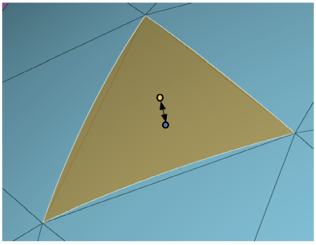
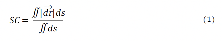
The surface element deviation is the integration of the difference between the mesh surface and the geometry surface over the surface triangular or quadrilateral element. Equation (1) integrates the distance from a mesh node to the geometry over the surface of an element using numerical integration and results in the average distance between the mesh and the surface.

The distance given by |dr| is the surface element deviation, as described in the Surface Element Deviation section. 
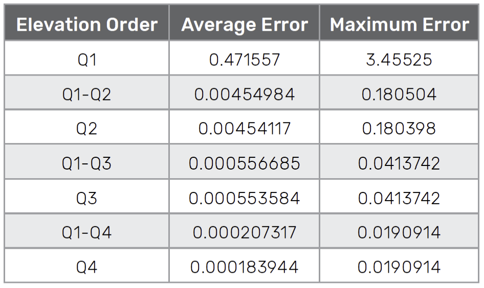
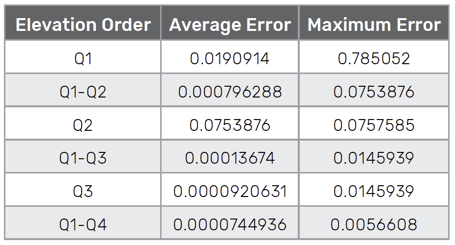
The shape conformity metric produces a dimensional quantity in the units of the mesh length scale. For flat planar surfaces, all mesh orders should produce machine zero values, indicating the mesh is on the planar surface. For curved boundaries, the linear mesh should exhibit the largest error, and increasing the mesh order should produce smaller error values.


Volume Element Deviation
 

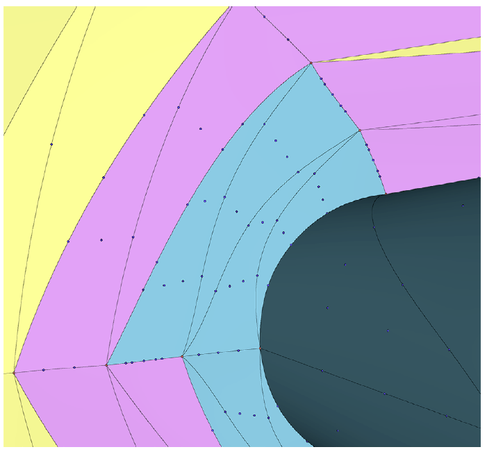
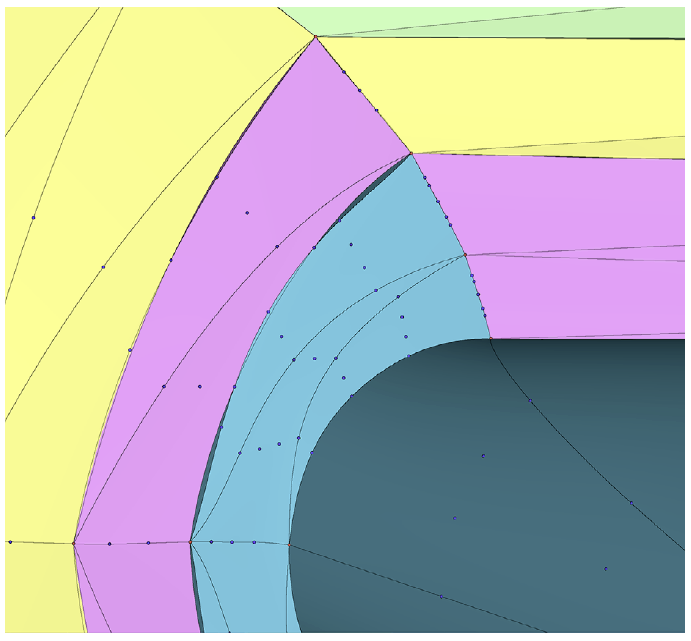
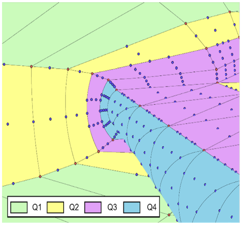
Volume elements with neighbors of a different order need deviation testing to ensure the shapes at the interface are similar. As illustrated in Figure 3a, the high-order nodes on the face common to elements of different order are not shared by each element, which can result in gaps at the interface. The deviation test is performed at these interfaces in one of two ways: either testing the lower order nodes against the higher order shape, or vice versa.

(a)
(b)

When performing mesh smoothing, the nodes on the faces and edges of the lower-order element are projected onto he adjacent higher-order shape. For instance, at the interface between a cubic and a quartic element, the nodes on the cubic element are forced to adhere to the quartic shape. The same is true for nodes at the interface of the Q3 and Q2 elements. Linear (Q1) elements have no face interior
or edge interior nodes, so no shape enforcement is required.
Periodically, during mesh smoothing, the deviation test is performed where the nodes on the higher-order side are tested against the lower order shape. The parametric coordinates of the higher order nodes are used to compute the physical coordinates on the lower order shape, using the lower order basis function and physical nodes. If the distance from the current location to the lower order shape location exceeds the deviation threshold, then the lower order element at that interface is marked for elevation.
When the two shapes at element interfaces converge within the tolerance, p-refinement stops. At the completion of mesh smoothing, before export, the higher-order nodes at these mixed-order interfaces are projected (not just measured) to the lower-order shapes, as illustrated in Figure 3b.


Results


Two realistic, complex cases are included that demonstrate the ability of the WCN-based mesh curving approach: the juncture flow model (JFM) and the NASA high-lift common research model (CRM-HL).


JFM


The juncture flow model (JFM) is a popular case for validating CFD methods on wing root viscous separation. It is the focus of numerous studies and workshops, including the 3rd American Institute of Aeronautics and Astronautics (AIAA) Geometry and Mesh Generation Workshop (GMGW-3) [2]. A mixed-order mesh family was generated for this workshop, the coarsest level of which is shown in Figure 4a. 

Cubic elements are shown on the highest curvature regions of the body, while some elements on the flat portion of the fuselage remain linear. The highest curvature in the geometry occurs at the wing tip trailing edge, shown in Figure 4b. The wing tip is rounded, and the coarse grid shown here has only four elements wrapped around a 180-degree turn near the trailing edge. At the completion of each mesh smoothing phase, the shape conformity metric is evaluated for all boundaries except planar boundaries, such as symmetry planes. The error values achieved for the shape conformity metric for the JFM fuselage are listed in Table 1. As expected, the errors reduce significantly as the element order is increased. Notice that the maximum error for the mixed-order Q1-Q3 and uniform-order Q3 meshes are equal. The same is true for the Q1-Q4 and Q4 meshes.

(a)
(b)
Figure 4: Mixed-order meshes of the JFM – (a) Full view showing Q1-Q3 elements, (b) Cut at the wing tip trailing edge showing mixed-order Q1-Q4 elements.

This indicates that the maximum error occurs on an element of maximum order, Q3 and Q4, respectively. The average error difference between the mixed and fully elevated orders for the same maximum order mesh only varies slightly. This is expected with the user-specified deviation metric of 0.01. Smaller values of the deviation metric will reduce this difference further at the cost of elevating more elements in the mesh to the higher order.

Table 1: Shape Conformity for JFM Fuselage
Table 2: Shape Conformity for JFM Wing

CRM-HL


Another case studied at GMGW-3 was the NASA High Lift Common Research Model (CRM-HL) configuration. This case was the focus of the 4th AIAA High Lift Prediction Workshop (HLPW-4) [3] co-located with GMGW-3. A mixed-order mesh family was also generated for this configuration. The meshes shown below represent the coarsest level meshes from the sequence. The symmetry plane mesh is mostly linear, as shown in Figure 5a. The center section of the fuselage is quadratic. Cubic and quartic elements are shown for the forward and aft fuselage regions. Most of the underside of the wing, shown in Figure 5c, is quadratic. Cubic and quartic elements exist at the leading edges of the wing and nacelle. This is also true for the topside view of the slats and nacelle pylon shown in Figure 5b. 

Figure 5: Mixed-order mesh of the CRM-HL using linear through quartic elements – (a) Symmetry plane, (b) Nacelle, (c) Underside of the wing

An axial cut at the wing tip trailing edge is shown in Figure 6a. This very coarse mesh has only two triangle elements spanning the 180-degree turn of the rounded wing tip. The wall-normal spacing, equivalent to an approximate Y+ value of 100, is extremely coarse. Much finer wall normal spacing was used for other meshes in the series, but those are more difficult to visualize. Also shown in the figure are the nodes of the mesh. Notice that the quartic elements contain five points (four segments) along each edge. When the adjacent element is cubic, these mid-edge nodes are not shared. The adjacent elements have a different set of edge internal points. The enforcement of shape conformity at this interface ensures that the curves represented on each side are the same, eliminating gaps in the mesh. A cut through the volume mesh at the engine nacelle/pylon is shown in Figure 6b. The high curvature of the nacelle leading edge is resolved with quartic elements. Quadratic elements cover most of the nacelle. The majority of the elements away from the curved geometry remain linear.

Figure 6: Cutting planes showing Q1-Q4 elements on the CRM-HL – (a) Axial cut at wing tip trailing edge, (b) Cut at engine nacelle and pylon
Conclusion
 

A method for generating curved, mixed-order meshes has been presented. Geometry access is provided through the MeshLink API. A deviation metric is used to indicate when surface and volume elements need elevation. Elements up to the fourth order are possible. Iterative perturbation-based smoothing ensures that a valid, high-quality mesh is produced. The cost function for the smoothing is comprised of a normalized Jacobian component that ensures positive Jacobians and a WCN component that enforces element shape. The combination allows for the elevation and smoothing of meshes, including clustering to viscous boundaries. Shape conformity is imposed between elements of a different order and used to evaluate the error between the elevated surface mesh and the underlying geometry. Two examples of realistic geometries were presented for configurations studied at HLPW-4 and GMGW-3.

References
1. Computational geometry kernel support. U.S. Air Force contract FA9101-18-P-0042, Topic AF181-015
2. 3rd AIAA Geometry and Mesh Generation Workshop (GMGW-3). https://www.gmgworkshop.com
3. 4th AIAA High Lift Prediction Workshop (HLPW-4). https://hiliftpw.larc.nasa.gov/index-workshop4.htm

Do you want to elevate CFD Simulations to new heights? Discover Fidelity Pointwise and request a free trial today.